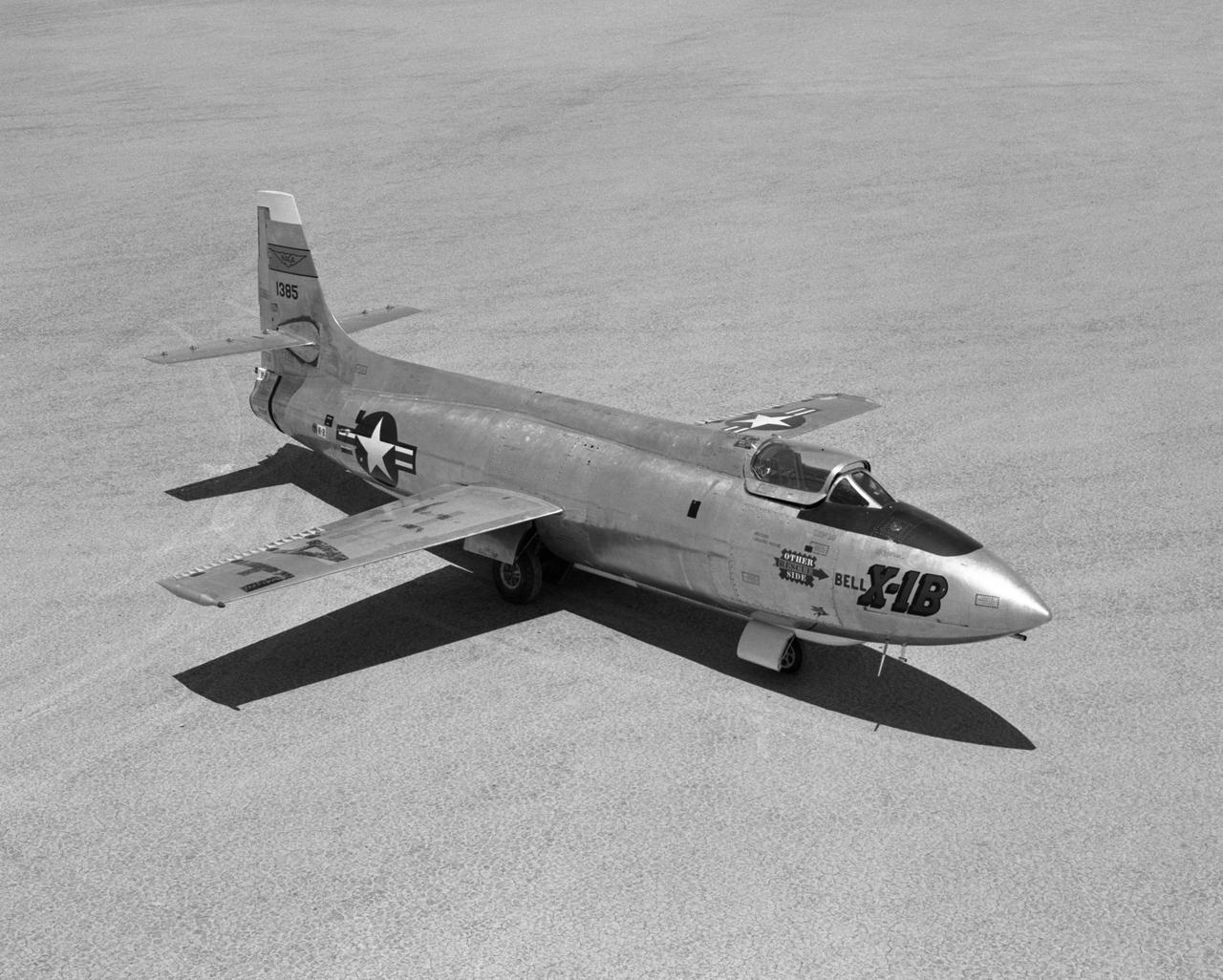
Bell X-1B fitted with a reaction control system on the lakebed
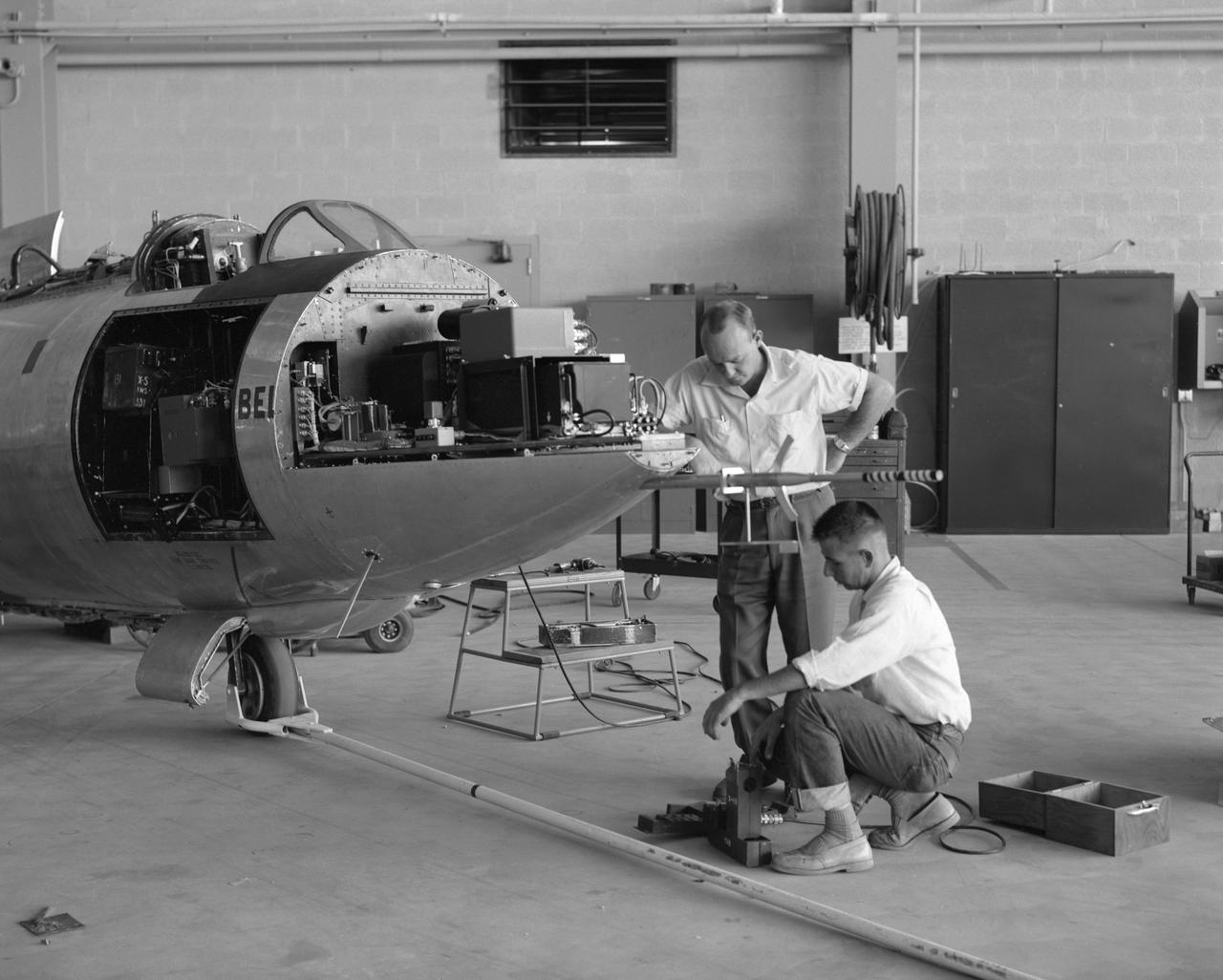
Lee Adelsbach and Bob Cook work on the instrumentation on the Bell X-1B.
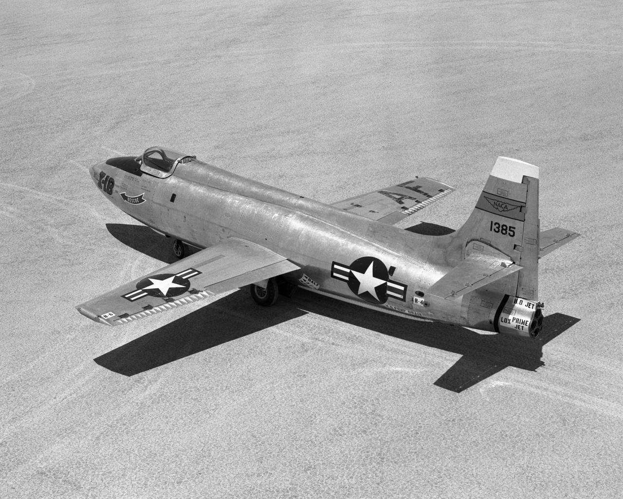
Bell X-1B fitted with a reaction control system on the lakebed.
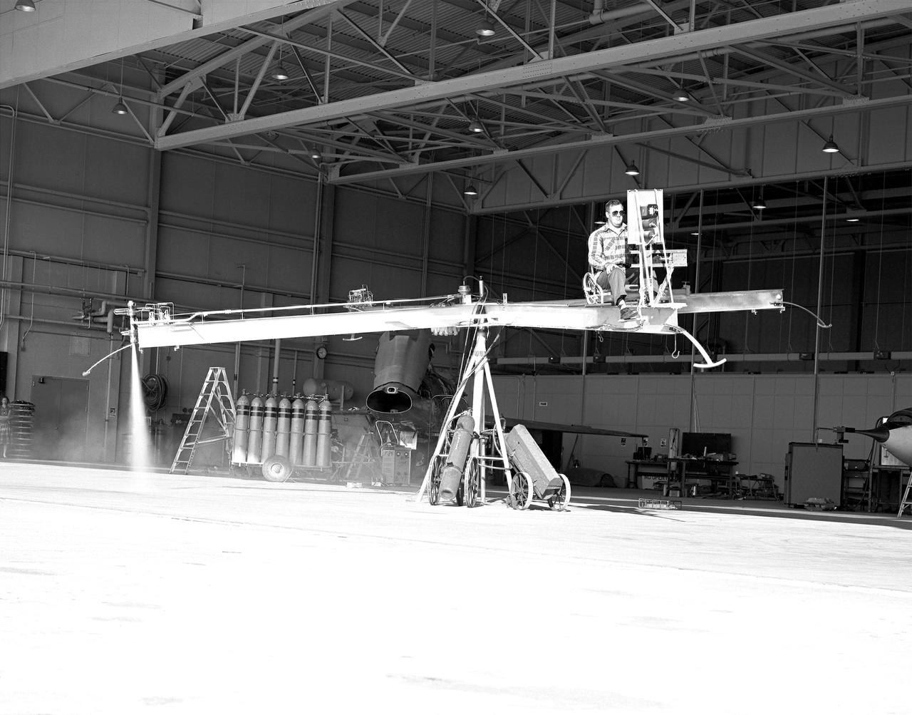
NACA High-Speed Flight Station test pilot Stan Butchart flying the Iron Cross, the mechanical reaction control simulator. High-pressure nitrogen gas expanded selectively, by the pilot, through the small reaction control thrusters maneuvered the Iron Cross through the three axes. The exhaust plume can be seen from the aft thruster. The tanks containing the gas can be seen on the cart at the base of the pivot point of the Iron Cross. NACA technicians built the iron-frame simulator, which matched the inertia ratios of the Bell X-1B airplane, installing six jet nozzles to control the movement about the three axes of pitch, roll, and yaw.
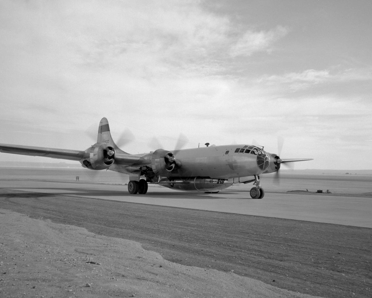
B-29 #800 with X-1B attached taxis in off of the lakebed.

B-29 #800 with X-1B attached taxi's in off of the lakebed.
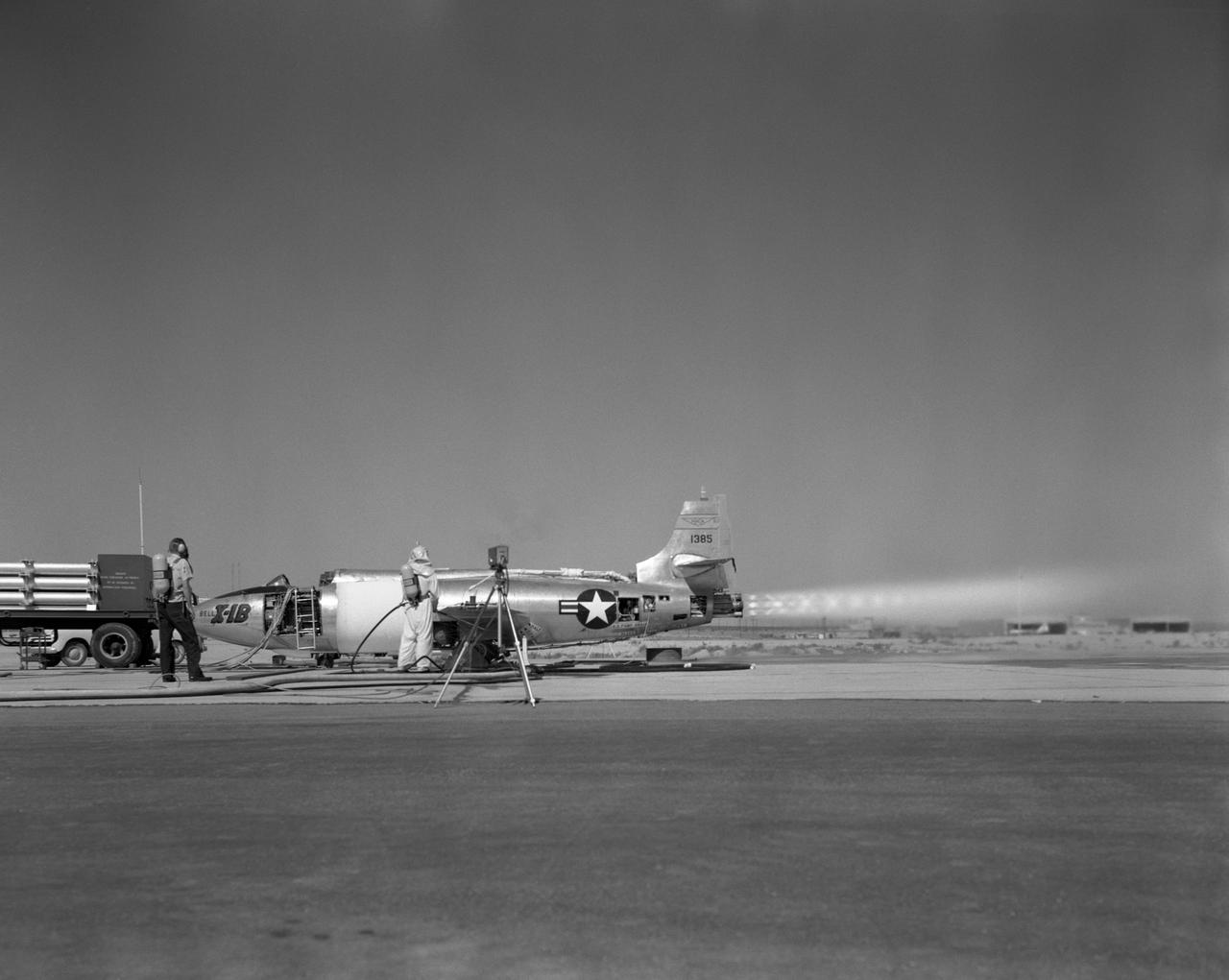
X-1B engine run on Air Force thrust stand.
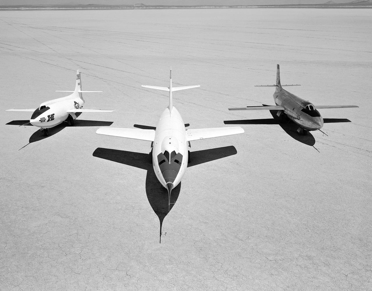
Early NACA research aircraft on the lakebed at the High Speed Research Station in 1955: Left to right: X-1E, D-558-II, X-1B
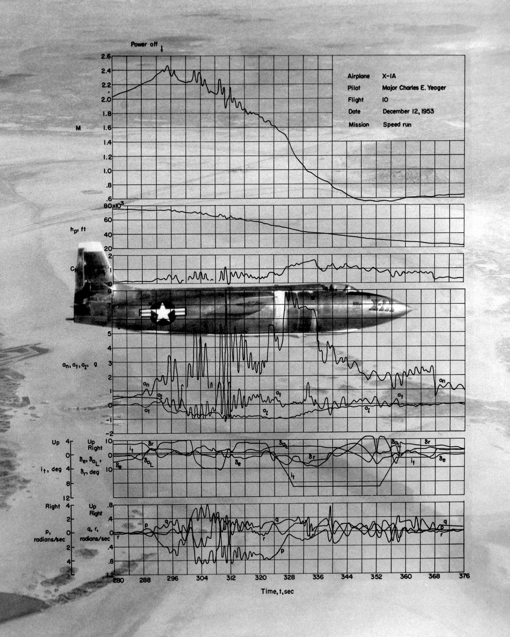
This photo of the X-1A includes graphs of the flight data from Maj. Charles E. Yeager's Mach 2.44 flight on December 12, 1953. (This was only a few days short of the 50th anniversary of the Wright brothers' first powered flight.) After reaching Mach 2.44, then the highest speed ever reached by a piloted aircraft, the X-1A tumbled completely out of control. The motions were so violent that Yeager cracked the plastic canopy with his helmet. He finally recovered from a inverted spin and landed on Rogers Dry Lakebed. Among the data shown are Mach number and altitude (the two top graphs). The speed and altitude changes due to the tumble are visible as jagged lines. The third graph from the bottom shows the G-forces on the airplane. During the tumble, these twice reached 8 Gs or 8 times the normal pull of gravity at sea level. (At these G forces, a 200-pound human would, in effect, weigh 1,600 pounds if a scale were placed under him in the direction of the force vector.) Producing these graphs was a slow, difficult process. The raw data from on-board instrumentation recorded on oscillograph film. Human computers then reduced the data and recorded it on data sheets, correcting for such factors as temperature and instrument errors. They used adding machines or slide rules for their calculations, pocket calculators being 20 years in the future.